The ArcGIS Content development team has (and still does!) put a lot of work into creating a comprehensive set of basemaps to help you as an ArcGIS user to show off your work, but, much as we would like to, we can’t cover everyone’s unique requirements. Until now, this effort was put into creating cached raster tile maps, but we are now expanding that by re-creating these maps in the new vector tile environment. One of the great features of vector tile mapping is that you now have the opportunity to customize the maps yourself. The extent to which you wish to do this is up to you, from ‘tweaking’ a few significant colors to creating a completely new look.
Three previous posts on the topic of Esri Vector Basemaps were recently published to the ArcGIS Blog: Introducing Esri Vector Basemaps (Beta), How to Customize Esri Vector Basemaps, and Customize Esri Vector Basemap Boundaries and Labels. Each post provides basic information for getting started to use and customize the vector basemap styles. This post builds on these and explores three more topics: JSON Structure, Inclusion, and Design.* It explains some basic controls you need to understand as you start stylizing your own vector basemaps. There is an Esri Vector Basemap Reference Document that includes lists of the map features with their label subtypes and min/max zoom levels and the list of disputed boundary codes.
JSON STRUCTURE
The root.JSON file controls the map style. For vector tile layers you own, you can downloaded the root.JSON, modify it, and update the item through ArcGIS.com. Having a good understanding of the JSON file structure will benefit you as you make modifications. This graphic highlights basic Esri Vector Basemap JSON code structure. On the right is a high-level list of features included in the maps (Background, Bathymetry, Land Use, etc.). The middle section details the type of feature (fill, stroke, etc.). The orange items have a fill and/or stroke symbol while the green items are labels and/or road shield symbols. Just as the lines of JSON code starts with map features in the background, the vector map draws these background features first followed by water fill, water lines, and roads, and completes by displaying road names, road shields, and city labels last. Keeping this general organization of the code in mind will help as you restyle the map.

INCLUSION
Whether or not a feature is included at a specific scale or zoom level is controlled initially by our ArcGIS Pro Project. Consequently, if a feature is not already included in the document it cannot be added from our data. However, you can exclude an existing feature by scale using:
“minzoom” :* “” **where the value is the smallest zoom level at which you want the feature to appear, and…
“maxzoom” :* “”* *where the value is the largest zoom level at which you want the feature to appear.
A full list of map features and their associated min/max zoom levels is included in the vector tile reference document.
A feature can be removed completely from the map (at all scales) by adding a visibility line to the “layout” command:
“layout” : {“visibility” : “none”},
Don’t forget to find and remove the equivalent label item if you are removing a feature from the map.
DESIGN
Dramatic changes can be made to the appearance of a basemap just by manipulating color and line widths. We will focus on those adjustments now.
Color
Styling instructions are controlled by the “paint” command, and this includes color. Here is an example:
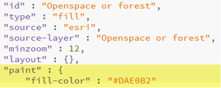
The color is a ‘HEX’ value, which in this case is a pale green

The RGB value for this color is: R218 G224 B178. If you are not used to working in HEX there are simple converters available online that will provide you with the equivalent to any RGB value.
To add an outline to a polygon, add another line item in the “paint” command:
“fill-outline-color” :* “#”
To adjust the opacity of your polygon, add
“fill-opacity” :* “” to the “paint” command. This works as a simple ratio, where ’0′ is completely transparent, and ’1′ is completely opaque.
Some of the current symbolization uses imported ‘sprites’ to generate a pattern effect. These are added to the “paint” command using:* “fill-pattern” :* “”
Lines
Here is an example of a line symbol:
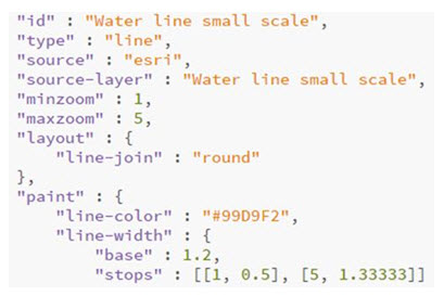
Line width is included in the ‘paint’ command and is measured in points. In this case the “base” value is set at 1.2 pts.
“stops” are added to vary the line width by scale or zoom level. In this case at Zoom 1 the line width is half of the “base” – 0.6pts. At Zoom 5, the line width is 1.33 times the base, or 1.6pts. The line width will adjust progressively between these stops, and you can add more stops if you wish.
To add a dash pattern to your line, add
“line-dasharray” :* [ 3.0 , 2.0 ] to the “paint” command. In this case, ’3.0′ is the length of the dash, and ’2.0′ is the interval between. Currently only a simple dash can be generated.
To adjust the opacity of your line, add
“line-opacity” : *”” to the “paint” command. As with the fill command, this works as a simple ratio, where ’0′ is completely transparent, and ’1′ is completely opaque.
These code modifications are the first steps for customizing the Esri Vector Basemap to your own map style.
Three previous posts on the topic of Esri Vector Basemaps were recently published to the ArcGIS Blog: Introducing Esri Vector Basemaps (Beta), How to Customize Esri Vector Basemaps, and Customize Esri Vector Basemap Boundaries and Labels. Each post provides basic information for getting started to use and customize the vector basemap styles. This post builds on these and explores three more topics: JSON Structure, Inclusion, and Design.* It explains some basic controls you need to understand as you start stylizing your own vector basemaps. There is an Esri Vector Basemap Reference Document that includes lists of the map features with their label subtypes and min/max zoom levels and the list of disputed boundary codes.
JSON STRUCTURE
The root.JSON file controls the map style. For vector tile layers you own, you can downloaded the root.JSON, modify it, and update the item through ArcGIS.com. Having a good understanding of the JSON file structure will benefit you as you make modifications. This graphic highlights basic Esri Vector Basemap JSON code structure. On the right is a high-level list of features included in the maps (Background, Bathymetry, Land Use, etc.). The middle section details the type of feature (fill, stroke, etc.). The orange items have a fill and/or stroke symbol while the green items are labels and/or road shield symbols. Just as the lines of JSON code starts with map features in the background, the vector map draws these background features first followed by water fill, water lines, and roads, and completes by displaying road names, road shields, and city labels last. Keeping this general organization of the code in mind will help as you restyle the map.
INCLUSION
Whether or not a feature is included at a specific scale or zoom level is controlled initially by our ArcGIS Pro Project. Consequently, if a feature is not already included in the document it cannot be added from our data. However, you can exclude an existing feature by scale using:
“minzoom” :* “” **where the value is the smallest zoom level at which you want the feature to appear, and…
“maxzoom” :* “”* *where the value is the largest zoom level at which you want the feature to appear.
A full list of map features and their associated min/max zoom levels is included in the vector tile reference document.
A feature can be removed completely from the map (at all scales) by adding a visibility line to the “layout” command:
“layout” : {“visibility” : “none”},
Don’t forget to find and remove the equivalent label item if you are removing a feature from the map.
DESIGN
Dramatic changes can be made to the appearance of a basemap just by manipulating color and line widths. We will focus on those adjustments now.
Color
Styling instructions are controlled by the “paint” command, and this includes color. Here is an example:
The color is a ‘HEX’ value, which in this case is a pale green
The RGB value for this color is: R218 G224 B178. If you are not used to working in HEX there are simple converters available online that will provide you with the equivalent to any RGB value.
To add an outline to a polygon, add another line item in the “paint” command:
“fill-outline-color” :* “#”
To adjust the opacity of your polygon, add
“fill-opacity” :* “” to the “paint” command. This works as a simple ratio, where ’0′ is completely transparent, and ’1′ is completely opaque.
Some of the current symbolization uses imported ‘sprites’ to generate a pattern effect. These are added to the “paint” command using:* “fill-pattern” :* “”
Lines
Here is an example of a line symbol:
Line width is included in the ‘paint’ command and is measured in points. In this case the “base” value is set at 1.2 pts.
“stops” are added to vary the line width by scale or zoom level. In this case at Zoom 1 the line width is half of the “base” – 0.6pts. At Zoom 5, the line width is 1.33 times the base, or 1.6pts. The line width will adjust progressively between these stops, and you can add more stops if you wish.
To add a dash pattern to your line, add
“line-dasharray” :* [ 3.0 , 2.0 ] to the “paint” command. In this case, ’3.0′ is the length of the dash, and ’2.0′ is the interval between. Currently only a simple dash can be generated.
To adjust the opacity of your line, add
“line-opacity” : *”” to the “paint” command. As with the fill command, this works as a simple ratio, where ’0′ is completely transparent, and ’1′ is completely opaque.
These code modifications are the first steps for customizing the Esri Vector Basemap to your own map style.